Note
Go to the end to download the full example code.
Model
import shap
import numpy as np
import pandas as pd
import matplotlib.pyplot as plt

import xgboost as xgb
from xgboost import XGBRegressor

from ai4water import Model
from ai4water.utils.utils import TrainTestSplit
from ai4water.postprocessing import ProcessPredictions
from ai4water.postprocessing import PartialDependencePlot

from sklearn.model_selection import LearningCurveDisplay, ShuffleSplit

from utils import prepare_data, SAVE
from utils import set_rcParams
from utils import evaluate_model
from utils import regression_plot
from utils import residual_plot
from utils import print_version_info
from utils import bar_pie
print_version_info()
python 3.12.7 (main, Nov  5 2024, 16:16:58) [GCC 11.4.0]
os posix
ai4water 1.07
xgboost 2.1.3
easy_mpl 0.21.4
SeqMetrics 2.0.0
torch 2.5.1+cu124
numpy 1.26.4
pandas 1.5.3
matplotlib 3.8.4
sklearn 1.3.1
xarray 2024.3.0
netCDF4 1.7.2
seaborn 0.13.2
bnlearn 0.10.2
Script Executed on:  Wed Jan  1 06:32:07 2025
tot_cpus 2
avail_cpus 2
mem_gib 7.612831115722656
shap.initjs()
<IPython.core.display.HTML object>
set_rcParams()
data, cat_encoder, an_encoder = prepare_data()
print(data.shape)
(1044, 15)
print(data.columns)
Index(['Catalyst type', 'Surface area', 'Pore volume', 'BandGap (eV)', 'Au',
       'Bi', 'Fe', 'O', 'Catalyst loading (g/L)', 'Light intensity (W)',
       'time (min)', 'solution pH', 'Anions', 'Ci (mg/L)', 'Efficiency (%)'],
      dtype='object')
TrainX, TestX, TrainY, TestY = (TrainTestSplit(seed=313).
                                split_by_random(data.iloc[:,0:-1], data.iloc[:,-1]))
print(TrainX.shape)
(730, 14)
print(TrainY.shape)
(730,)
print(TestX.shape)
(314, 14)
print(TestY.shape)
(314,)
model = Model(model='XGBRegressor',
              cross_validator={"KFold": {'n_splits': 50}}
              )
building ML model for
regression problem using XGBRegressor
model.fit(TrainX, TrainY)
# fig, ax = plt.subplots(figsize=(30, 30))
# xgb.plot_tree(model._model, ax=ax)
# plt.savefig('../manuscript/figures/figS2.png', dpi=600, bbox_inches="tight")
# plt.show()
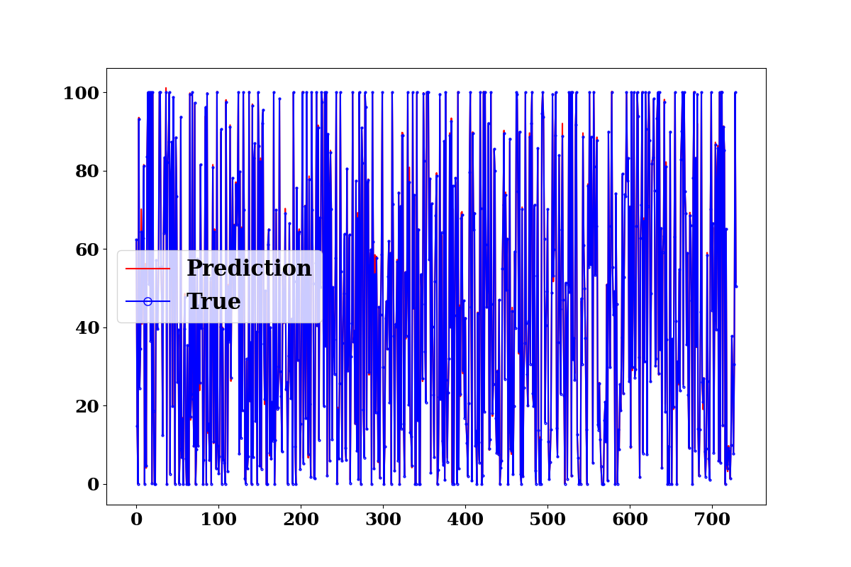
train_p = model.predict(TrainX)
evaluate_model(TrainY.values, train_p)
mse 0.7981642712436582
rmse 0.8934003980543428
r2 0.9993237665126041
r2_score 0.9993236785411198
mape inf
mae 0.4882864061401118
processor = ProcessPredictions('regression', forecast_len=1,
                               plots=['prediction'])

processor(TrainY.values, train_p)
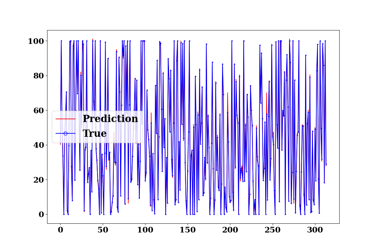
test_p = model.predict(TestX)
evaluate_model(TestY.values, test_p)
mse 3.538625835769641
rmse 1.8811235567526237
r2 0.9969561205228433
r2_score 0.9969450676175826
mape inf
mae 0.9911163492994325
processor = ProcessPredictions('regression', forecast_len=1,
                               plots=['prediction'])

processor(TestY.values, test_p)
set_rcParams({'xtick.labelsize': '14',
'ytick.labelsize': '14'})
pp = ProcessPredictions('regression', 1, show=False)
common_params = {
"X": data.iloc[:,0:-1],
"y": data.iloc[:,-1],
"train_sizes": np.linspace(0.1, 1.0, 5),
"cv": ShuffleSplit(n_splits=50, test_size=0.2, random_state=0),
"score_type": "both",
'scoring':'neg_mean_squared_error',
"n_jobs": 4,
"line_kw": {"marker": "o"},
"std_display_style": "fill_between",
"score_name": "MSE",
}
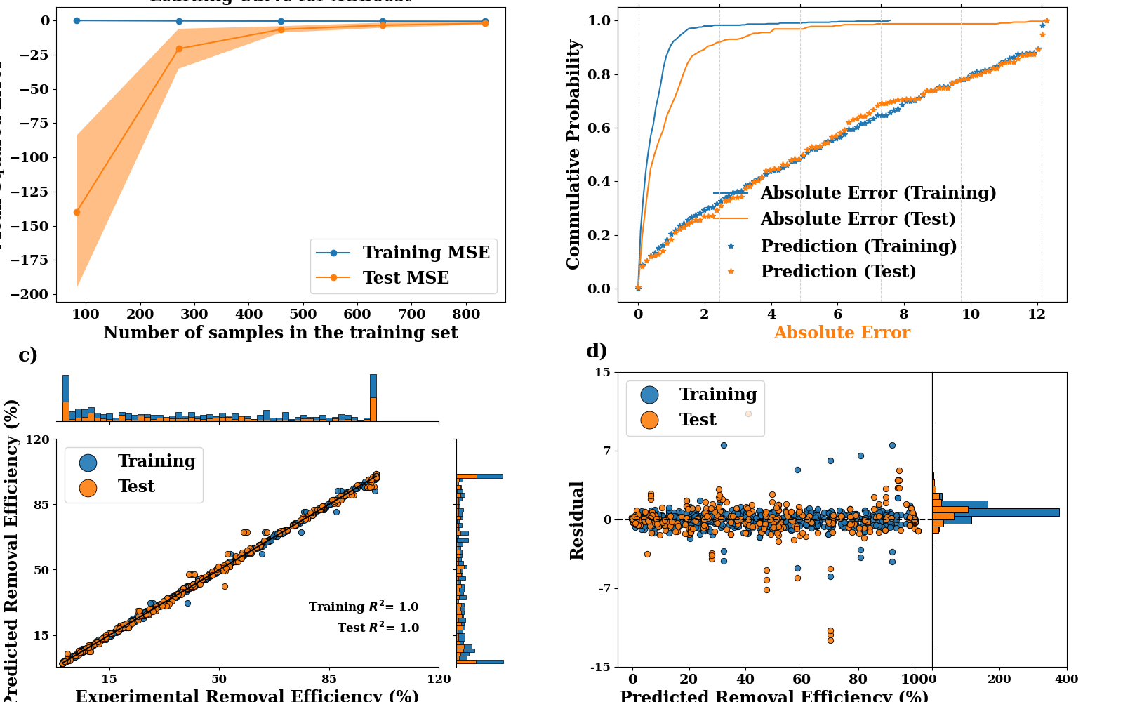
# Create figure with specified aspect ratio
fig = plt.figure(figsize=(16, 10))
# Manually set the axes positions [left, bottom, width, height]
# These values are normalized (0 to 1) relative to the figure size
ax1 = fig.add_axes([0.05, 0.57, 0.4, 0.42]) # First row, first two columns
ax2 = fig.add_axes([0.55, 0.57, 0.4, 0.42]) # First row, last two columns
ax3 = fig.add_axes([0.05, 0.05, 0.4, 0.42]) # Second row, first two columns
ax4 = fig.add_axes([0.55, 0.05, 0.28, 0.42]) # Second row, third and part of fourth columns
ax5 = fig.add_axes([0.83, 0.05, 0.12, 0.42]) # Second row, last column
ax1.text(-0.1, 1.05, 'a)', transform=ax1.transAxes, size=20, weight='bold')
ax2.text(-0.1, 1.05, 'b)', transform=ax2.transAxes, size=20, weight='bold')
ax3.text(-0.1, 1.34, 'c)', transform=ax3.transAxes, size=20, weight='bold')
ax4.text(-0.1, 1.05, 'd)', transform=ax4.transAxes, size=20, weight='bold')
# Remove y-ticks from the fifth axis
ax5.set_yticks([])
#for ax_idx, estimator in enumerate([naive_bayes, svc]):
LearningCurveDisplay.from_estimator(XGBRegressor(), **common_params, ax=ax1)
handles, label = ax1.get_legend_handles_labels()
ax1.legend(handles[:2], ["Training MSE", "Test MSE"], fontsize=17, loc='lower right')
ax1.set_title(f"Learning Curve for XGBoost", fontsize=17)
ax1.set_xlabel("Number of samples in the training set", fontsize=17)
ax1.set_ylabel("Mean Squared Error", fontsize=17)
# **** EDF plot
output = pp.edf_plot(TrainY.values, train_p,
ax=ax2,
color=('tab:blue', 'tab:blue'),
marker=('-', '*'),
label=("Absolute Error (Training)", "Prediction (Training)"))
output = pp.edf_plot(TestY.values, test_p,
marker=('-', '*'),
ax=output[0], pred_axes=output[1],
color=('tab:orange', 'tab:orange'),
label=("Absolute Error (Test)", "Prediction (Test)"))
output[0].legend(loc=(0.20, 0.23), frameon=False, fontsize=17)
output[1].legend(loc=(0.20, 0.05), frameon=False, fontsize=17)
output[0].set_xlabel('Absolute Error', fontsize=17)
output[1].set_xlabel('Prediction', fontsize=17)
output[0].set_ylabel('Commulative Probability', fontsize=17)
# **** Regression plot
ax3 = regression_plot(TrainY.values, train_p, TestY.values, test_p, ax=ax3,
train_color='tab:blue', test_color='tab:orange')
ax3.set_xlim(-2, ax3.get_xlim()[1])
ax3.set_ylim(-2, ax3.get_ylim()[1])
ax3.set_ylabel("Predicted Removal Efficiency (%)", fontsize=17)
ax3.set_xlabel("Experimental Removal Efficiency (%)", fontsize=17)
ax3.legend(loc='upper left', markerscale=3, fontsize=17)
# **** Residual plot
axis = residual_plot(
TrainY.values,
train_p,
TestY.values,
test_p,
label="Efficiency",
axis=(ax4, ax5),
train_color='tab:blue',
test_color='tab:orange',
)
axis[0].set_ylabel("Residual", fontsize=17)
axis[0].set_xlabel("Predicted Removal Efficiency (%)", fontsize=17)
axis[0].legend(loc='upper left', markerscale=3, fontsize=17)
#plt.savefig("../manuscript/figures/fig4.png", dpi=600, bbox_inches="tight")
# Show the plot
plt.show()
SHAP
explainer = shap.Explainer(model._model, TrainX)

shap_values = explainer(TrainX)

type(shap_values)
print(shap_values.shape)
(730, 14)
CATEGORIES = {
    'Experimental Conditions':
        ["Ci (mg/L)", "time (min)", "solution pH", "Anions", "Light intensity (W)", "Catalyst loading (g/L)", "Anions", "Catalyst type"],
    'Physiochemical Properties':
        ['Pore volume', 'Surface area', 'BandGap (eV)'],
    'Atomic Composition':
        ['Bi', 'O', 'Fe', 'Au'],
          }

def make_classes(exp):
    colors = {
          'Experimental Conditions': '#405f77',
          'Physiochemical Properties': '#1fafd2',
          'Atomic Composition': '#f2826e',
          }

    classes = []
    colors_ = []
    for f in exp.feature_names:
        if f in CATEGORIES['Experimental Conditions']:
            classes.append('Experimental Conditions')
            colors_.append(colors['Experimental Conditions'])
        elif f in CATEGORIES['Physiochemical Properties']:
            classes.append('Physiochemical Properties')
            colors_.append(colors['Physiochemical Properties'])
        elif f in CATEGORIES['Atomic Composition']:
            classes.append('Atomic Composition')
            colors_.append(colors['Atomic Composition'])
        else:
            raise ValueError(f"{f} not found")

    return classes, colors_

sv_bar = np.mean(np.abs(shap_values.values), axis=0)

classes, colors_ = make_classes(shap_values)

df_with_classes = pd.DataFrame(
    {'features': shap_values.feature_names,
     'classes': classes,
     'mean_shap': sv_bar,
     'colors': colors_
     })

print(df_with_classes)

ax, *_= bar_pie(df_with_classes,
         save=False,
         name="bar_pie",
         pie_pos="center",
        show=False)

# remove right spine
ax.spines['right'].set_visible(False)
ax.spines['top'].set_visible(False)
#plt.savefig('../manuscript/figures/fig5.png', dpi=600, bbox_inches="tight")
plt.show()
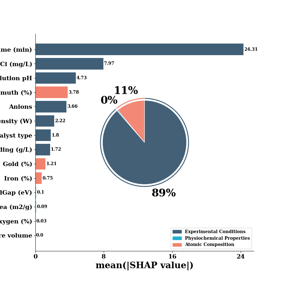
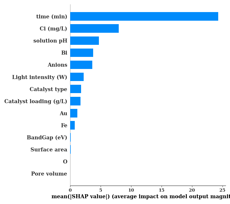
                  features                    classes  mean_shap   colors
0            Catalyst type    Experimental Conditions   1.804110  #405f77
1             Surface area  Physiochemical Properties   0.091180  #1fafd2
2              Pore volume  Physiochemical Properties   0.000000  #1fafd2
3             BandGap (eV)  Physiochemical Properties   0.095963  #1fafd2
4                       Au         Atomic Composition   1.206869  #f2826e
5                       Bi         Atomic Composition   3.784539  #f2826e
6                       Fe         Atomic Composition   0.754104  #f2826e
7                        O         Atomic Composition   0.026943  #f2826e
8   Catalyst loading (g/L)    Experimental Conditions   1.721145  #405f77
9      Light intensity (W)    Experimental Conditions   2.220205  #405f77
10              time (min)    Experimental Conditions  24.306885  #405f77
11             solution pH    Experimental Conditions   4.729943  #405f77
12                  Anions    Experimental Conditions   3.657640  #405f77
13               Ci (mg/L)    Experimental Conditions   7.968859  #405f77
Experimental Conditions 0.8861985591113752
Physiochemical Properties 0.0035735825030922927
Atomic Composition 0.11022785838553249
shap.summary_plot(shap_values, TrainX.values,
                  plot_type="bar",
                  feature_names=data.columns[0:-1], show=False)

if SAVE:
    plt.savefig('figures/shap_bar.png')
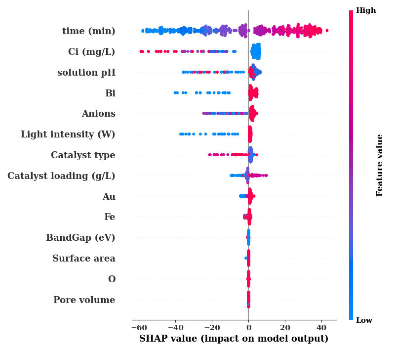
shap.summary_plot(shap_values, TrainX.values,
                  feature_names=data.columns[0:-1], show=False)

if SAVE:
    plt.savefig('figures/shap.png')
sample_id = 0

print(shap_values.base_values[sample_id] + shap_values[sample_id].values.sum())

shap.plots.force(shap_values[sample_id],
                matplotlib=True,
                plot_cmap="LpLb",
                #  show=False
                 )
61.74045086603148
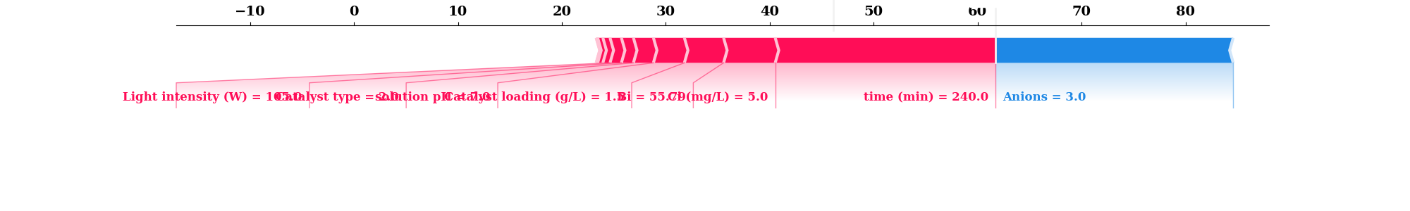
sample with maximum shap value
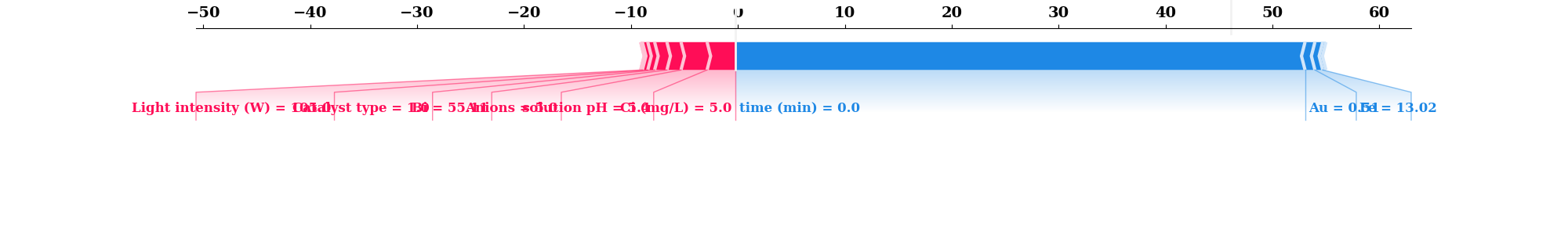
sample_id = np.argmax(shap_values.values.sum(axis=1))
print(sample_id, shap_values.base_values[sample_id] + shap_values[sample_id].values.sum())

shap_values.values[sample_id][10] = 26.03

figure = shap.plots.force(shap_values[sample_id],
                matplotlib=True,
                plot_cmap="LpLb",
                show=False,
                figsize=(24, 4)
                 )

#plt.savefig('../manuscript/figures/fig6a.png', dpi=600, bbox_inches="tight")
36 101.16288013871878
sample with minimum shap value
sample_id = np.argmin(shap_values.values.sum(axis=1))
print(sample_id, shap_values.base_values[sample_id] + shap_values[sample_id].values.sum())

shap.plots.force(shap_values[sample_id],
                matplotlib=True,
                plot_cmap="LpLb",
                #  show=False
                 )
85 -0.22594724009073275
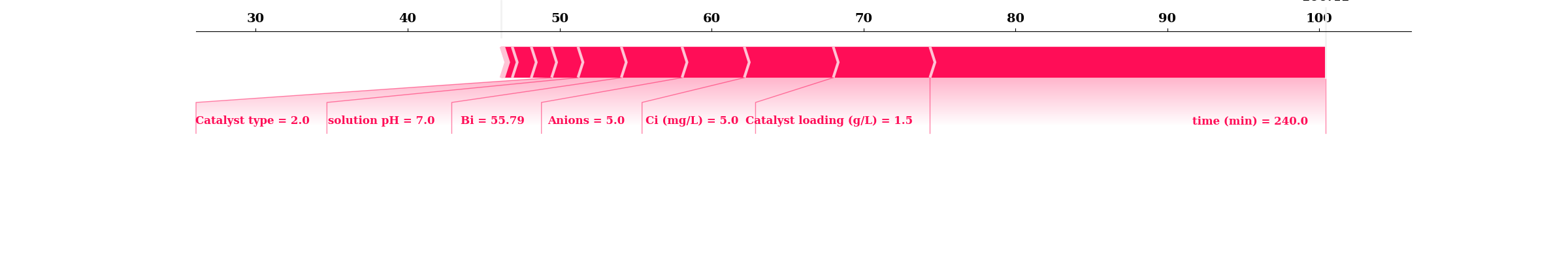
sample with second minimum shap value
sample_id = np.argsort(shap_values.values.sum(axis=1))[80]
print(sample_id, shap_values.base_values[sample_id] + shap_values[sample_id].values.sum())

shap.plots.force(shap_values[sample_id],
                matplotlib=True,
                plot_cmap="LpLb",
                show=False,
                figsize=(24, 4)
                 )
#plt.savefig('../manuscript/figures/fig6b.png', dpi=600, bbox_inches="tight")
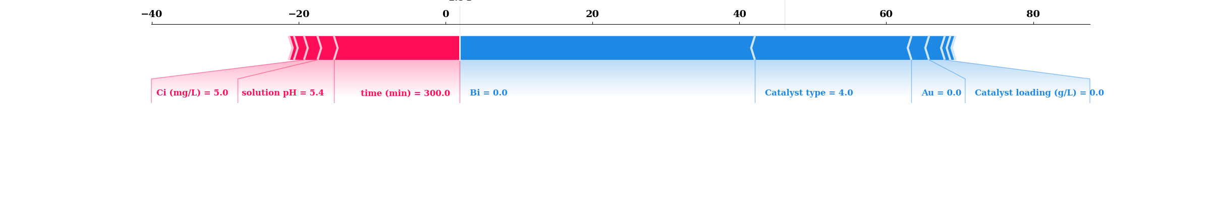
470 1.938715847813107

<Figure size 2400x400 with 1 Axes>
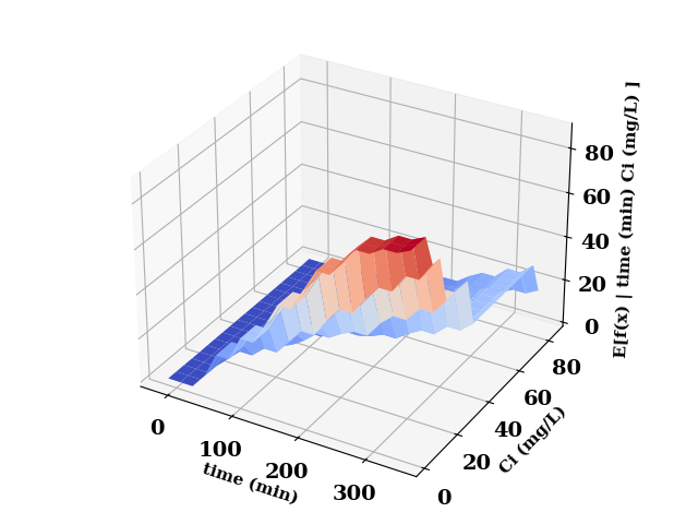
Partial Dependence Plot
pdp = PartialDependencePlot(
    model.predict,
    TrainX,
    num_points=20,
    feature_names=list(TrainX.columns),
    show=False,
    save=False
)
pdp.plot_interaction(
    features=['time (min)', 'Ci (mg/L)'],
    plot_type="surface",
    cmap="coolwarm",
)
plt.tight_layout()
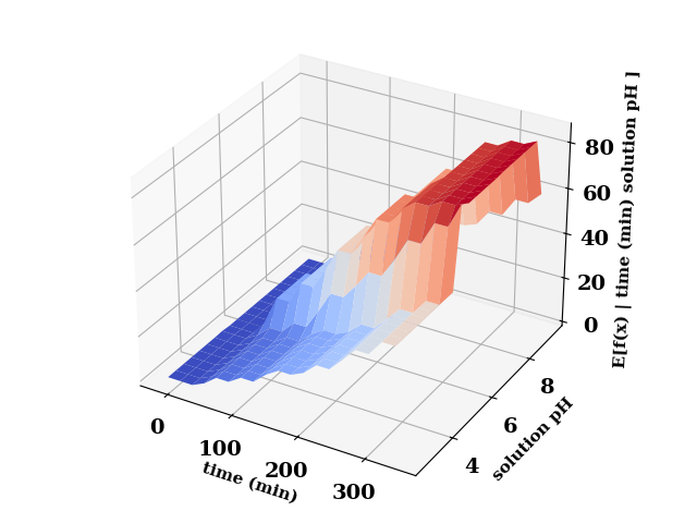
pdp.plot_interaction(
    features=['time (min)', 'solution pH'],
    plot_type="surface",
    cmap="coolwarm",
)
plt.tight_layout()
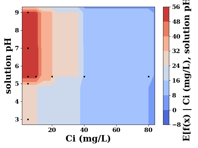
pdp.plot_interaction(
    features=['Ci (mg/L)', 'solution pH'],
    plot_type="contour",
    cmap="coolwarm",
)
plt.tight_layout()
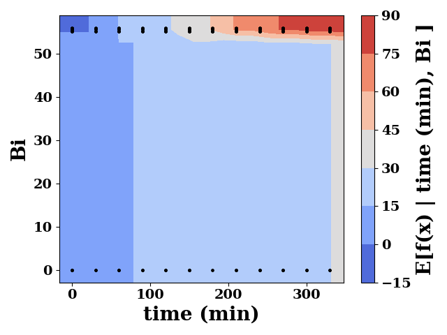
ax = pdp.plot_interaction(
    features=['time (min)', 'Bi'],
    plot_type="contour",
    cmap="coolwarm",
)
plt.tight_layout()
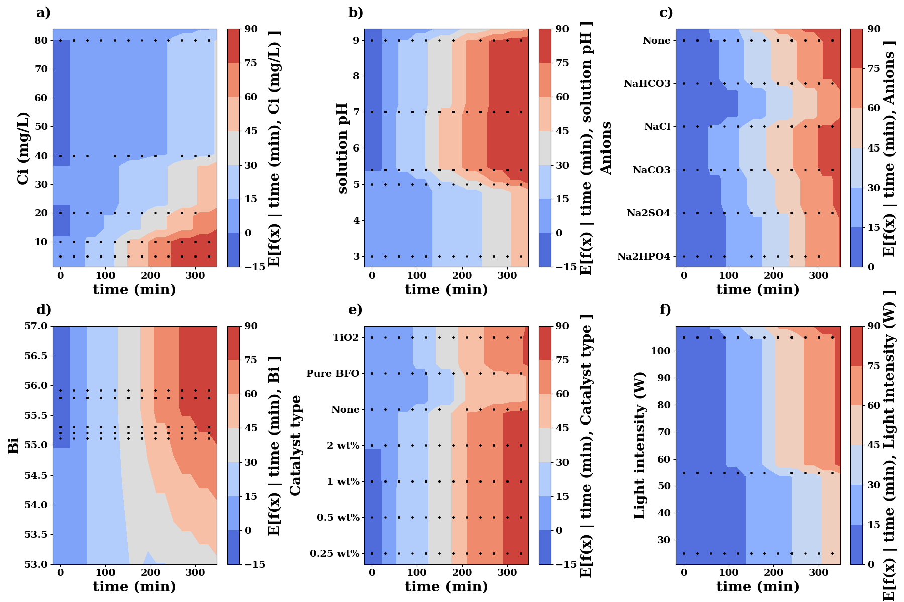
f, ((ax1, ax2, ax3), (ax4, ax5, ax6)) = plt.subplots(2, 3, figsize=(18, 12))

pdp.plot_interaction(
    features=['time (min)', 'Ci (mg/L)'],
    plot_type="contour",
    cmap="coolwarm",
    ax=ax1,
)
ax1.text(-0.1, 1.05, 'a)', transform=ax1.transAxes, size=20, weight='bold')

pdp.plot_interaction(
    features=['time (min)', 'solution pH'],
    plot_type="contour",
    cmap="coolwarm",
    ax=ax2,
)
ax2.text(-0.1, 1.05, 'b)', transform=ax2.transAxes, size=20, weight='bold')

ax = pdp.plot_interaction(
    features=['time (min)', 'Anions'],
    plot_type="contour",
    cmap="coolwarm",
    ax=ax3,
)
anions = [0, 1, 2, 3, 4, 5]
ax.set_yticks(range(len(anions)))
ax.set_yticklabels(an_encoder.inverse_transform(anions))
ax3.text(-0.1, 1.05, 'c)', transform=ax3.transAxes, size=20, weight='bold')

ax = pdp.plot_interaction(
    features=['time (min)', 'Bi'],
    plot_type="contour",
    cmap="coolwarm",
    ax=ax4,
)
ax.set_ylim(53, 57)
ax4.text(-0.1, 1.05, 'd)', transform=ax4.transAxes, size=20, weight='bold')

ax = pdp.plot_interaction(
    features=['time (min)', 'Catalyst type'],
    plot_type="contour",
    cmap="coolwarm",
    ax=ax5,
)
catalysts = [0, 1, 2, 3, 4, 5, 6]
ax.set_yticks(range(len(catalysts)))
ax.set_yticklabels(cat_encoder.inverse_transform(catalysts))
ax5.text(-0.1, 1.05, 'e)', transform=ax5.transAxes, size=20, weight='bold')

pdp.plot_interaction(
    features=['time (min)', 'Light intensity (W)'],
    plot_type="contour",
    cmap="coolwarm",
    ax=ax6,
)
ax6.text(-0.1, 1.05, 'f)', transform=ax6.transAxes, size=20, weight='bold')

plt.tight_layout()
#plt.savefig('../manuscript/figures/fig7.png', dpi=600, bbox_inches="tight")
plt.show()
Total running time of the script: (0 minutes 30.475 seconds)