Note
Go to the end to download the full example code.
Exploratory Data Analysis
import os
import pandas as pd

import matplotlib.pyplot as plt

from easy_mpl import imshow
from easy_mpl.utils import create_subplots

from mne.viz import circular_layout
from mne_connectivity.viz import plot_connectivity_circle

from utils import SAVE
from utils import LABEL_MAP
from utils import set_rcParams
from utils import distribution_plot
from utils import pie_from_series
from utils import merge_uniques
from utils import prepare_data
from utils import print_version_info
# Print the version info of the packages being used
print_version_info()
python 3.12.7 (main, Nov  5 2024, 16:16:58) [GCC 11.4.0]
os posix
ai4water 1.07
xgboost 2.1.3
easy_mpl 0.21.4
SeqMetrics 2.0.0
torch 2.5.1+cu124
numpy 1.26.4
pandas 1.5.3
matplotlib 3.8.4
sklearn 1.3.1
xarray 2024.3.0
netCDF4 1.7.2
seaborn 0.13.2
bnlearn 0.10.2
Script Executed on:  Wed Jan  1 06:31:55 2025
tot_cpus 2
avail_cpus 2
mem_gib 7.612831115722656
set_rcParams()
fpath = os.path.join("../data/data.xlsx")
df = pd.read_excel(fpath)
# Display the first 5 rows of the dataset
df.head()
Display the last 5 rows of the dataset
df.tail()
Display the shape of the dataset
df.shape
(1044, 16)
Display the columns of the dataset
df.columns
Index(['Catalyst type', 'Surface area', 'Pore volume', 'BandGap (eV)', 'Au',
       'Bi', 'Fe', 'O', 'Catalyst loading (g/L)', 'Light intensity (W)',
       'time (min)', 'solution pH', 'Anions', 'Ci (mg/L)', 'Cf (mg/L)',
       'Efficiency (%)'],
      dtype='object')
Display the info of the dataset
df.info()
<class 'pandas.core.frame.DataFrame'>
RangeIndex: 1044 entries, 0 to 1043
Data columns (total 16 columns):
 #   Column                  Non-Null Count  Dtype
---  ------                  --------------  -----
 0   Catalyst type           1044 non-null   object
 1   Surface area            1044 non-null   float64
 2   Pore volume             1044 non-null   float64
 3   BandGap (eV)            1044 non-null   float64
 4   Au                      1044 non-null   float64
 5   Bi                      1044 non-null   float64
 6   Fe                      1044 non-null   float64
 7   O                       1044 non-null   float64
 8   Catalyst loading (g/L)  1044 non-null   float64
 9   Light intensity (W)     1044 non-null   int64
 10  time (min)              1044 non-null   int64
 11  solution pH             1044 non-null   float64
 12  Anions                  1044 non-null   object
 13  Ci (mg/L)               1044 non-null   int64
 14  Cf (mg/L)               1044 non-null   float64
 15  Efficiency (%)          1044 non-null   float64
dtypes: float64(11), int64(3), object(2)
memory usage: 130.6+ KB
Display the summary statistics of the dataset
df.describe()
Display the missing values of the dataset
df.isnull().sum()
Catalyst type             0
Surface area              0
Pore volume               0
BandGap (eV)              0
Au                        0
Bi                        0
Fe                        0
O                         0
Catalyst loading (g/L)    0
Light intensity (W)       0
time (min)                0
solution pH               0
Anions                    0
Ci (mg/L)                 0
Cf (mg/L)                 0
Efficiency (%)            0
dtype: int64
Display the duplicated rows of the dataset
df.duplicated().sum()
218
numerical columns
num_columns = ['Surface area', 'Pore volume', 'BandGap (eV)', 'Au',
       'Bi', 'Fe', 'O', 'Catalyst loading (g/L)', 'Light intensity (W)',
       'time (min)', 'solution pH', 'Ci (mg/L)', 'Cf (mg/L)',
       'Efficiency (%)']
Display the distribution of the numerical columns
for col in num_columns:
    print(f"{col}: {df[col].describe()}")


data_num = df[num_columns].copy()
Surface area: count    1044.000000
mean       20.796552
std         6.395003
min         0.000000
25%        21.600000
50%        21.600000
75%        21.600000
max        45.000000
Name: Surface area, dtype: float64
Pore volume: count    1044.000000
mean        0.004038
std         0.000856
min         0.000000
25%         0.004300
50%         0.004300
75%         0.004300
max         0.004900
Name: Pore volume, dtype: float64
BandGap (eV): count    1044.000000
mean        2.314138
std         0.465941
min         0.000000
25%         2.350000
50%         2.350000
75%         2.350000
max         3.200000
Name: BandGap (eV), dtype: float64
Au: count    1044.000000
mean        0.887586
std         0.389551
min         0.000000
25%         1.000000
50%         1.000000
75%         1.000000
max         1.980000
Name: Au, dtype: float64
Bi: count    1044.000000
mean       51.886207
std        14.129589
min         0.000000
25%        55.790000
50%        55.790000
75%        55.790000
max        55.920000
Name: Bi, dtype: float64
Fe: count    1044.000000
mean       12.670000
std         3.455051
min         0.000000
25%        13.680000
50%        13.680000
75%        13.680000
max        13.680000
Name: Fe, dtype: float64
O: count    1044.000000
mean       27.651724
std         7.556266
min         0.000000
25%        29.520000
50%        29.520000
75%        29.520000
max        31.600000
Name: O, dtype: float64
Catalyst loading (g/L): count    1044.000000
mean        1.143678
std         0.425064
min         0.000000
25%         1.000000
50%         1.000000
75%         1.500000
max         2.500000
Name: Catalyst loading (g/L), dtype: float64
Light intensity (W): count    1044.000000
mean      100.517241
std        16.943329
min        25.000000
25%       105.000000
50%       105.000000
75%       105.000000
max       105.000000
Name: Light intensity (W), dtype: float64
time (min): count    1044.00000
mean      165.00000
std       103.61121
min         0.00000
25%        82.50000
50%       165.00000
75%       247.50000
max       330.00000
Name: time (min), dtype: float64
solution pH: count    1044.000000
mean        6.034483
std         1.104839
min         3.000000
25%         5.400000
50%         5.400000
75%         7.000000
max         9.000000
Name: solution pH, dtype: float64
Ci (mg/L): count    1044.000000
mean        9.482759
std        14.998264
min         5.000000
25%         5.000000
50%         5.000000
75%         5.000000
max        80.000000
Name: Ci (mg/L), dtype: float64
Cf (mg/L): count    1044.000000
mean        6.670795
std        14.254075
min         0.000000
25%         1.280000
50%         3.070000
75%         4.742500
max        80.000000
Name: Cf (mg/L), dtype: float64
Efficiency (%): count    1044.000000
mean       44.788506
std        34.274206
min         0.000000
25%        11.400000
50%        40.600000
75%        74.850000
max       100.000000
Name: Efficiency (%), dtype: float64
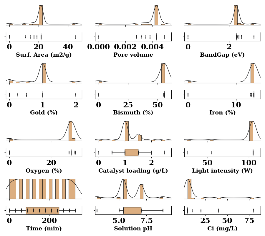
fig, axes = create_subplots(data_num.shape[1]-2, figsize=(9, 8))
for ax, col in zip(axes.flat, data_num.columns):
    if col in ['Cf (mg/L)', 'Efficiency (%)']:
        continue

    distribution_plot(ax=ax, data=data_num[col],
                      box_facecolor='#dcae80',
                      scatter_fc = '#1b1b1c',
                      ridge_lc='#1b1b1c',

                      )
    ax.set_xlabel(xlabel=LABEL_MAP.get(col, col), weight='bold', fontsize=14)
    ax.set_yticklabels('')
plt.tight_layout()

# plt.savefig("../manuscript/figures/fig2.png", dpi=600,
#             bbox_inches="tight")
plt.show()
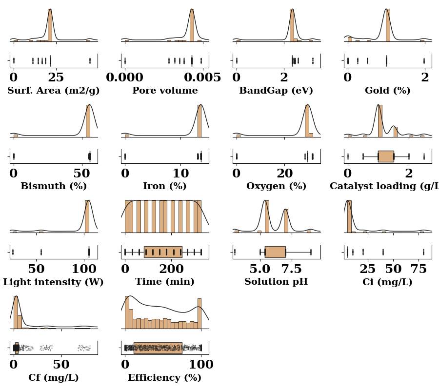
fig, axes = create_subplots(data_num.shape[1], figsize=(9, 8))
for ax, col in zip(axes.flat, data_num.columns):

    distribution_plot(ax=ax, data=data_num[col],
                      box_facecolor='#dcae80',
                      scatter_fc = '#1b1b1c',
                      ridge_lc='#1b1b1c',

                      )
    ax.set_xlabel(xlabel=LABEL_MAP.get(col, col), weight='bold', fontsize=14)
    ax.set_yticklabels('')
plt.tight_layout()

plt.show()
Categorical Data
categorical columns
cat_columns = ['Catalyst type', 'Anions']
Display the unique values of the categorical columns
for col in cat_columns:
    print(f"{col}: {df[col].unique()}")
Catalyst type: ['no catalyst' 'pure BFO' '0.25 wt% Au-BFO' '0.5 wt% Au-BFO'
 '1 wt% Au-BFO' '2 wt% Au-BFO' 'commercial TiO2']
Anions: ['Without Anions' 'NaCl' 'Na2SO4' 'NaCO3' 'NaHCO3' 'Na2HPO4']
Display the value counts of the categorical columns
for col in cat_columns:
    print(f"{col}: {df[col].value_counts()}")


merged_series = merge_uniques(df['Catalyst type'], 7)
pie_from_series(merged_series, cmap="coolwarm",  show=False, leg_pos=(0.85, 0.7))
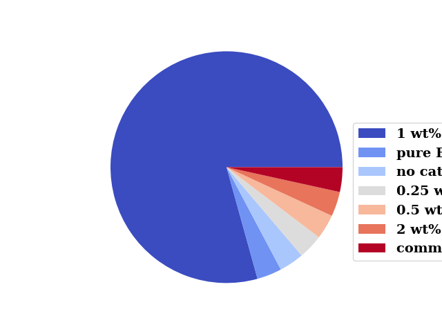
Catalyst type: 1 wt% Au-BFO 828
pure BFO 36
no catalyst 36
0.25 wt% Au-BFO 36
0.5 wt% Au-BFO 36
2 wt% Au-BFO 36
commercial TiO2 36
Name: Catalyst type, dtype: int64
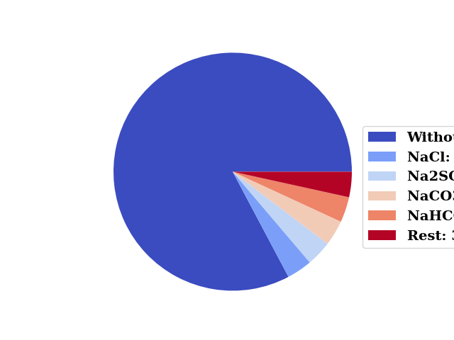
Anions: Without Anions 864
NaCl 36
Na2SO4 36
NaCO3 36
NaHCO3 36
Na2HPO4 36
Name: Anions, dtype: int64
merged_series = merge_uniques(df['Anions'], 5)
pie_from_series(merged_series, cmap="coolwarm",  show=False, leg_pos=(0.85, 0.7))
Correlation
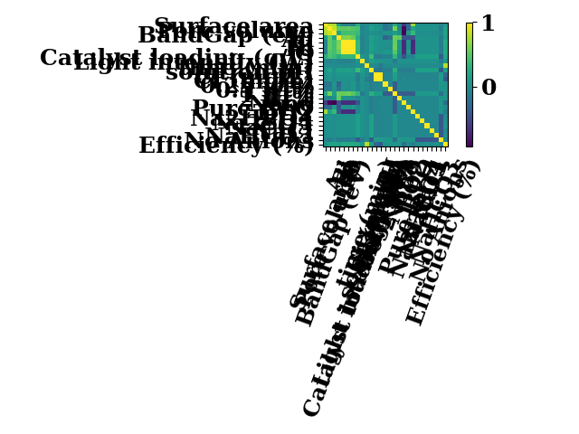
df, cat_enc, an_enc = prepare_data(encoding="ohe", exclude_cf=False)
df = df.rename(
    columns={f"Catalyst type_{idx}":category for idx, category in enumerate(cat_enc.categories_[0])})
df = df.rename(
    columns={f"Anions_{idx}":category for idx, category in enumerate(an_enc.categories_[0])})
# # %%

corr = df.corr(method="pearson")
imshow(corr, colorbar=True, show=False)
plt.tight_layout()
plt.show()
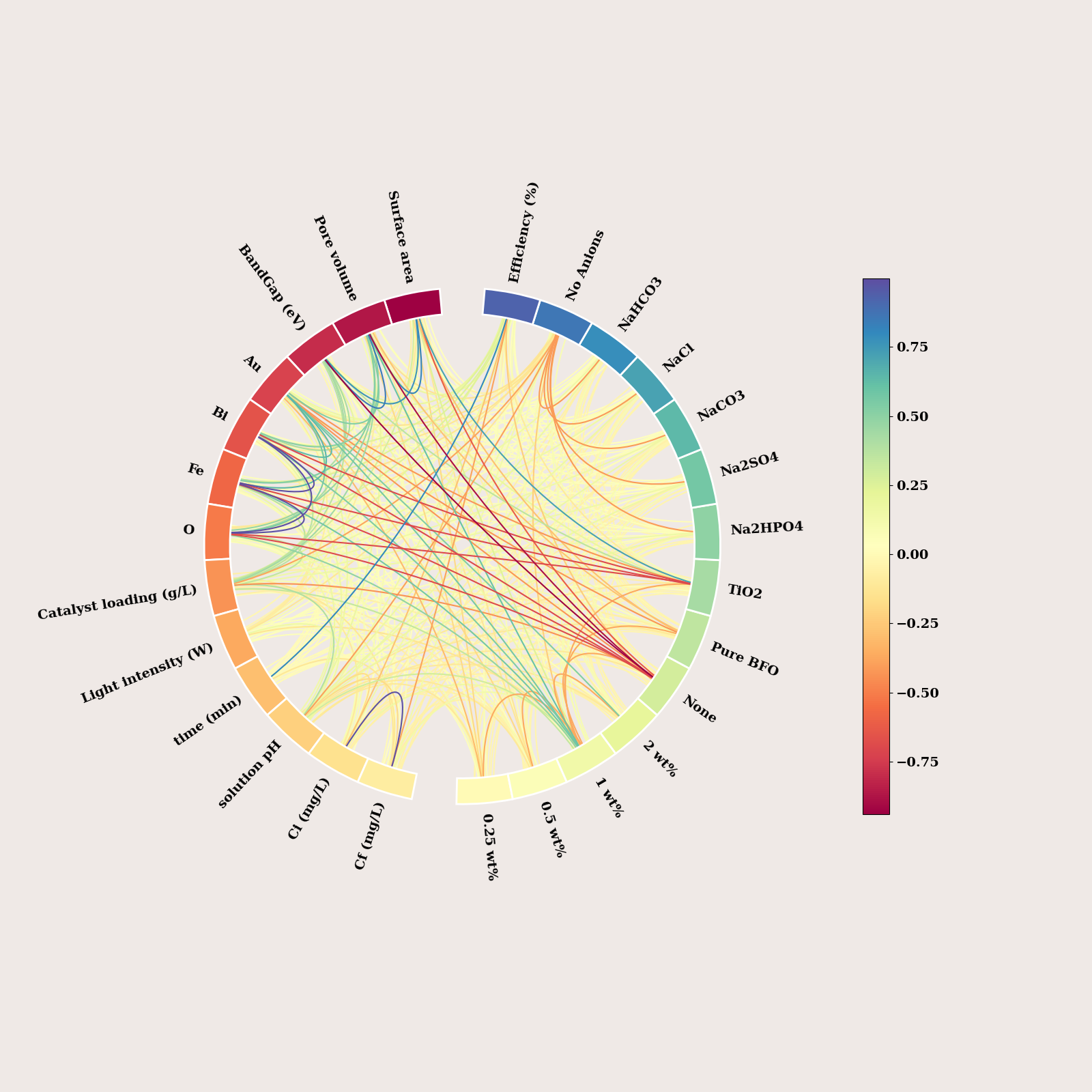
df = df.fillna(0.0)
node_angles = circular_layout(corr.columns.tolist(), corr.columns.tolist(),
                              start_pos=90, group_boundaries=[0, len(corr.columns.tolist()) // 2])

print(node_angles.shape)
(27,)
fig, ax = plt.subplots(figsize=(16, 16),
                       facecolor="#EFE9E6",
                       subplot_kw=dict(polar=True))
fig, axes = plot_connectivity_circle(
    corr.values,
    node_names = corr.columns.tolist(),
    node_angles=node_angles,
    fontsize_names =14,
    fontsize_colorbar =14,
    facecolor ="#EFE9E6",
    textcolor='black',
    #n_lines = 14,
    node_edgecolor="white",
    colormap="Spectral",
    colorbar_size=0.5,
    colorbar_pos=(-0.5, 0.5),
    ax=ax)

#fig.savefig(f"../manuscript/figures/fig3.png", dpi=600, bbox_inches="tight")
fig.tight_layout()
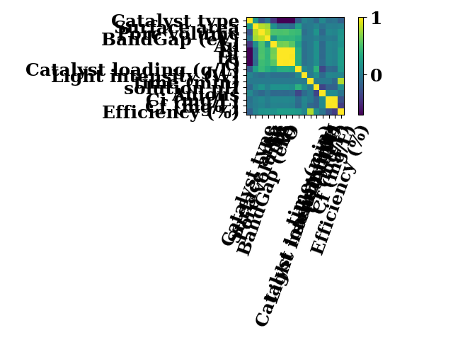
df, _, _ = prepare_data(encoding="le", exclude_cf=False)
corr = df.corr(method="pearson")
imshow(corr, colorbar=True, show=False)
plt.tight_layout()
plt.show()
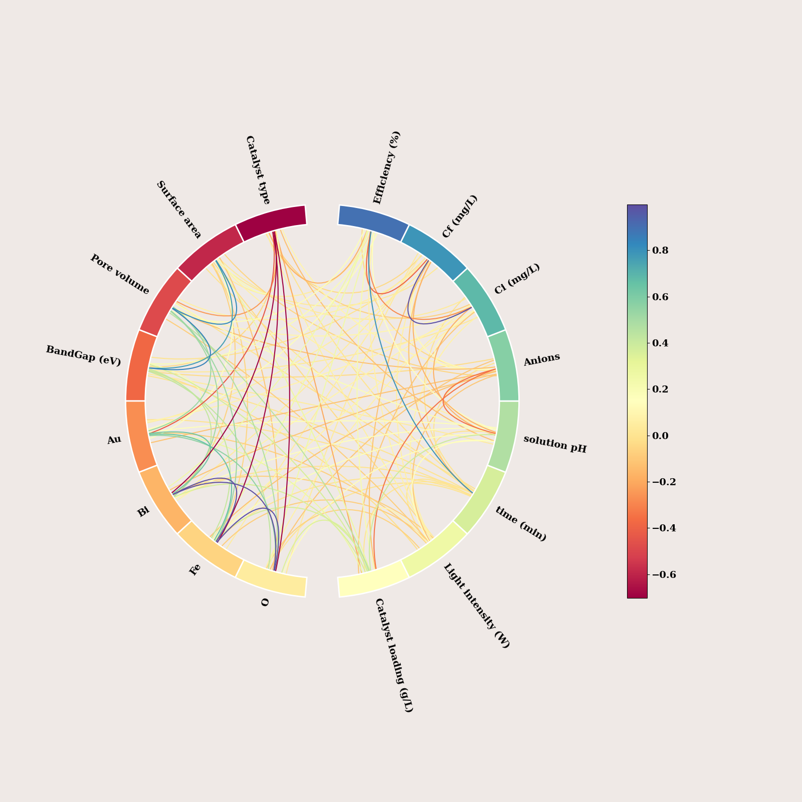
df = df.fillna(0.0)
node_angles = circular_layout(corr.columns.tolist(), corr.columns.tolist(),
                              start_pos=90, group_boundaries=[0, len(corr.columns.tolist()) // 2])

print(node_angles.shape)
(16,)
fig, ax = plt.subplots(figsize=(16, 16),
                       facecolor="#EFE9E6",
                       subplot_kw=dict(polar=True))
fig, axes = plot_connectivity_circle(
    corr.values,
    node_names = corr.columns.tolist(),
    node_angles=node_angles,
    fontsize_names =14,
    fontsize_colorbar =14,
    facecolor ="#EFE9E6",
    textcolor='black',
    #n_lines = 14,
    node_edgecolor="white",
    colormap="Spectral",
    colorbar_size=0.5,
    colorbar_pos=(-0.5, 0.5),
    ax=ax)

# fig.savefig(f"figures/chord_large_le", dpi=600, bbox_inches="tight")
fig.tight_layout()
df_org = pd.read_excel(fpath)
print(df_org.shape)
df_org = df_org.drop(columns=['Catalyst type', 'Anions'])
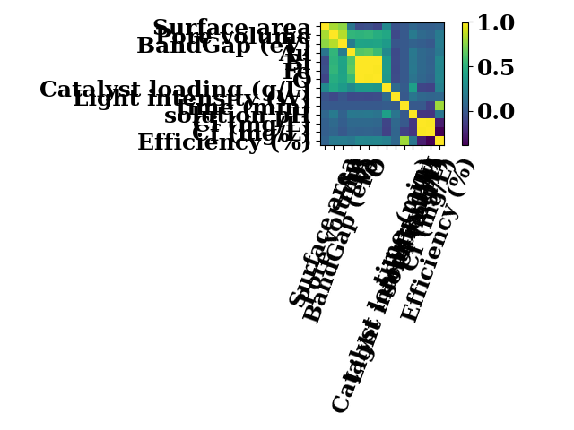
corr = df_org.corr(method="pearson")
imshow(corr, colorbar=True, show=False)
plt.tight_layout()
plt.show()
(1044, 16)
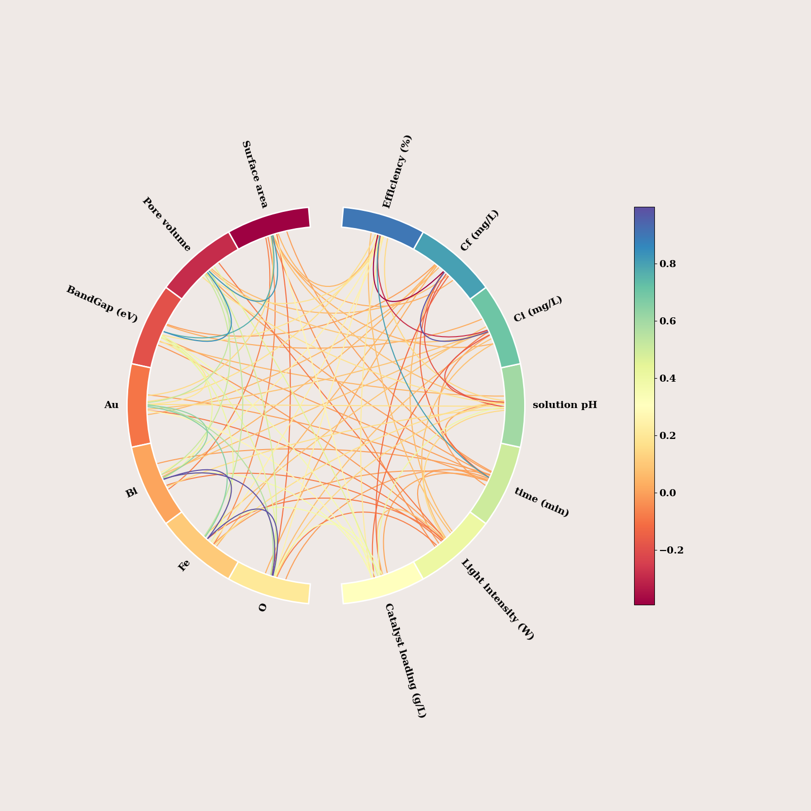
df_org = df_org.fillna(0.0)
node_angles = circular_layout(corr.columns.tolist(), corr.columns.tolist(),
                              start_pos=90, group_boundaries=[0, len(corr.columns.tolist()) // 2])

print(node_angles.shape)
(14,)
fig, ax = plt.subplots(figsize=(16, 16),
                       facecolor="#EFE9E6",
                       subplot_kw=dict(polar=True))
fig, axes = plot_connectivity_circle(
    corr.values,
    node_names = corr.columns.tolist(),
    node_angles=node_angles,
    fontsize_names =14,
    fontsize_colorbar =14,
    facecolor ="#EFE9E6",
    textcolor='black',
    #n_lines = 14,conda
    node_edgecolor="white",
    colormap="Spectral",
    colorbar_size=0.5,
    colorbar_pos=(-0.5, 0.5),
    ax=ax)

if SAVE:
    fig.savefig(f"figures/chord_large_org", dpi=600, bbox_inches="tight")
fig.tight_layout()
Total running time of the script: (0 minutes 11.910 seconds)